Paying Down the World-Model Tax: Latency Optimization for a Cosmos 3 Nano Policy

#NebiusServerlessChallenge

GitHub Repository

Robotics has been advancing rapidly, and many startups are trying to reach a “GPT-3 moment” for the field: a generalist model that performs well across many domains. Robot learning is harder than language modeling in several respects because it must combine capabilities such as understanding the environment, predicting actions, and acting in a 3D world. Many robotic systems still rely on a modular stack in which perception, planning, and control are designed or trained separately. A growing alternative is an end-to-end policy that maps instructions and observations directly to robot actions.

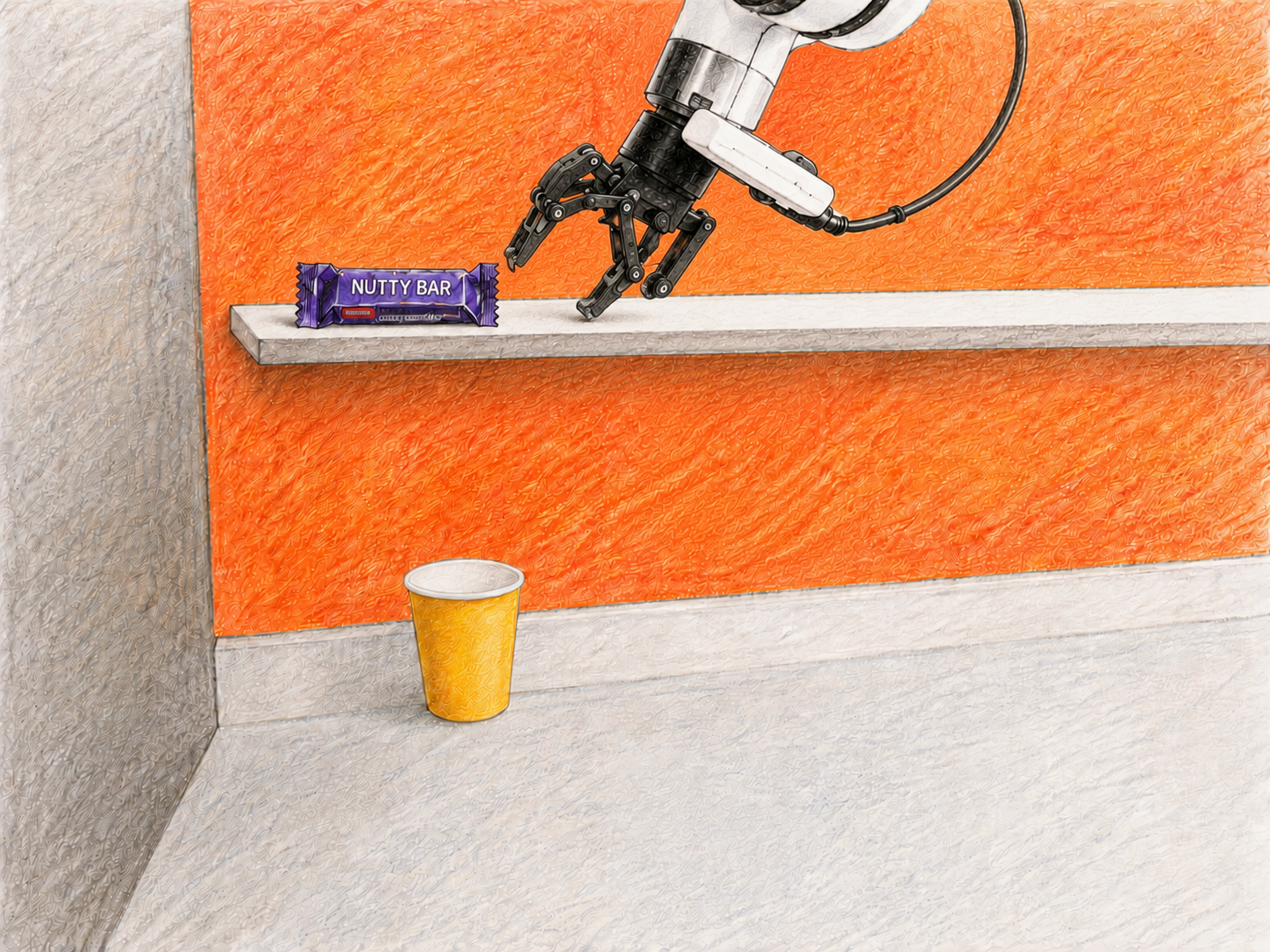
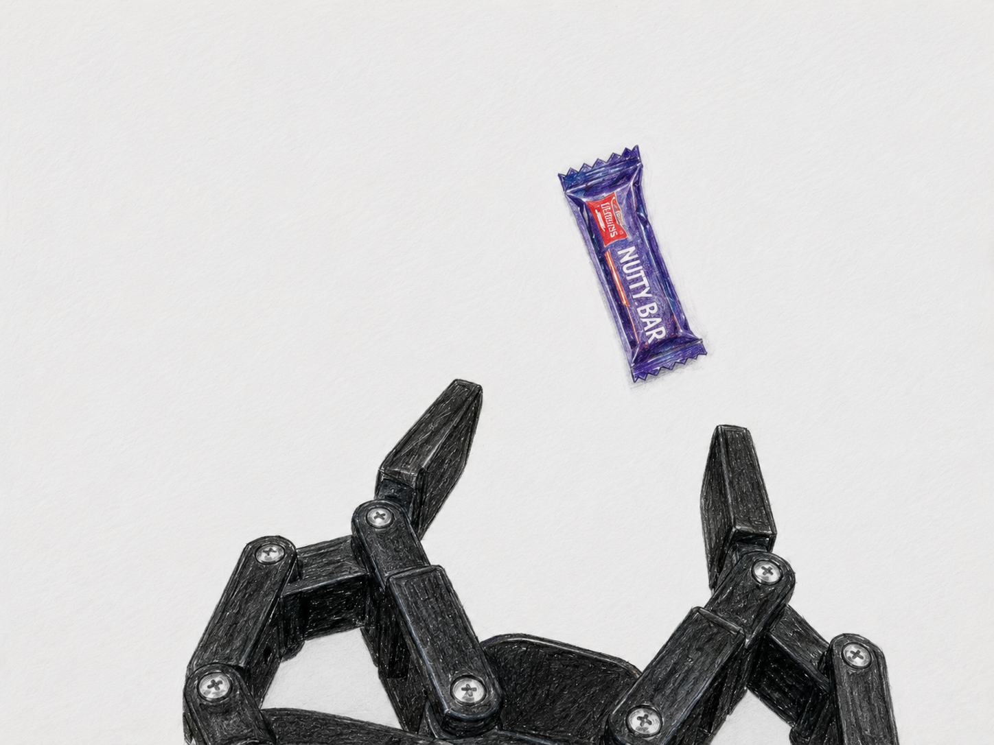
To illustrate, consider a robot that is asked to pick up a candy bar and place it on a shelf. The robot has cameras that provide views of the scene (in this example, three images), and it receives a natural-language instruction describing the task: “Put the candy bar on the left side of the first shelf.”

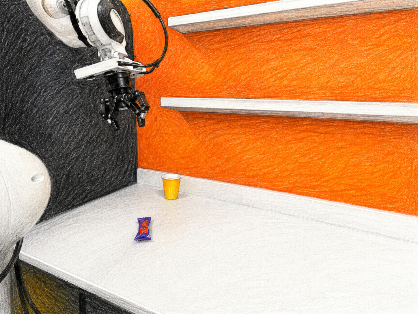
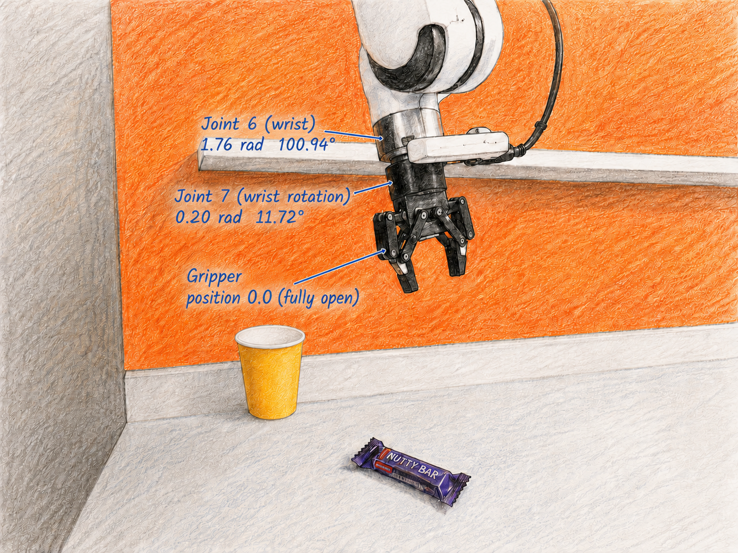
The robot also reports its own proprioceptive state—a short vector describing its current joint configuration, shown in the table and image below. From these inputs, the system has to produce the actions that complete the task.

Variable	Value	Angle	Location
joint 1	0.0858 rad	4.92°	base (lowest joint)
joint 2	−0.3002 rad	−17.20°	shoulder
joint 3	0.3066 rad	17.57°	upper arm
joint 4	−2.1223 rad	−121.60°	elbow
joint 5	−0.1432 rad	−8.20°	forearm
joint 6	1.7618 rad	100.94°	first wrist joint
joint 7	0.2046 rad	11.72°	final wrist / flange
Robotiq gripper	0.0	—	opening of the two black fingers

The system must understand the instruction, recognize the candy bar in the camera images, and plan movements that complete the task. One design uses separate models for these steps; another trains a single model to handle them jointly.

This single, general model is the goal. World-model approaches such as NVIDIA Cosmos 3 and DayDreamer, as well as vision-language-action models, or VLAs, such as NVIDIA Isaac GR00T, RT-2, OpenVLA, and π0, are important steps toward it. However, each robot embodiment has its own action space, including different joint configurations, gripper states, camera poses, and base controls. The Franka arm in the images above and a humanoid, for instance, do not expose the same control interface. As a result, these models generally need to be adapted or post-trained for the target embodiment and action representation.

This move toward more general and consequently larger models comes with additional costs. In Cosmos 3, the multimodal architecture increases latency as it requires more computation and memory traffic during inference. Moreover, the policy model generates actions through several diffusion steps, which adds even more latency.

Latency, alongside capability, determines whether a model is useful on a real robot. In this article, I examine the main contributors to the latency of a Cosmos 3 Nano policy released by NVIDIA at the end of May 2026 and techniques that can reduce it, together with the quality gate needed for lossy optimization.

World Models

As described above, robot learning has to solve three closely related tasks: understand the environment, decide what the robot should do, and optionally predict what will happen when it acts. A useful way to group current approaches is into three categories.

The first is action prediction. A policy model, such as a VLA, maps the observation history and a language instruction directly to a sequence of robot actions:

The second is future-state prediction, an idea that comes from the model-based reinforcement-learning and control tradition. An action-conditioned world model receives a proposed action sequence and predicts how the environment is likely to evolve:

The third approach combines both tasks. A world-action model predicts an action sequence together with its likely consequences:

In practice, the boundaries are less strict. Some policies use future-state prediction only during training, while some world-action models generate only actions at deployment. The Cosmos3-Nano-Policy-DROID checkpoint used in this article, for example, returns action trajectories even though the broader Cosmos 3 family can also model future observations.

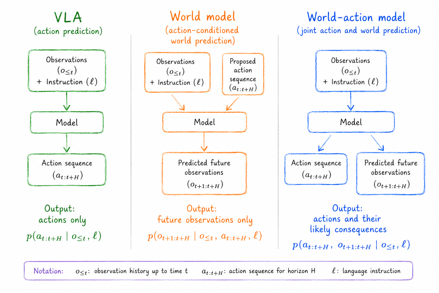
This still leaves an open question: what should the predicted “world” look like? It does not have to be a rendered image or video; it can also be structured object states, trajectories, or compact latent features.

Yann LeCun's JEPA line of work argues for prediction in an abstract latent space. I-JEPA, for example, predicts representations of masked regions in an image rather than reconstructing their pixels; V-JEPA extends representation prediction to video.

Fei-Fei Li and World Labs take a more explicit spatial-intelligence view. They believe that a world model should learn the structure of space and time well enough to reconstruct, generate, simulate, and update persistent interactive 3D environments.

NVIDIA's Cosmos 3 sits closer to the generative world-action end of this spectrum. It combines physical reasoning, world generation, and action generation within one model family. Depending on how it is post-trained, it can reason about observations, generate images or video, predict future states, or produce robot action sequences through a shared omnimodal architecture.

Cosmos 3 Overview

Cosmos 3 uses a Mixture-of-Transformers, or MoT, architecture. It combines two specialized transformer towers that process modalities including text, images, video, audio, and actions. For the robot example, one request carries the instruction, camera views, and robot state to a single policy model, which returns an action sequence. The two towers are called the Reasoner and the Generator.

The Reasoner processes text and images for scene understanding and physical reasoning. In the Nano and Super variants, it is an autoregressive vision-language model based on Qwen3-VL.

The Generator is diffusion-based. Conditioned on the Reasoner's "understanding", it generates continuous outputs such as images, video, audio, and action trajectories through iterative denoising.

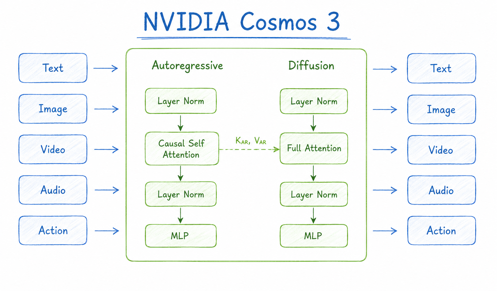
The Cosmos 3 technical report describes three sizes. Cosmos3-Super has 64 billion parameters and targets compute-heavy workloads such as synthetic-data generation and world simulation. Cosmos3-Nano has 16 billion parameters and is designed for more efficient inference. Cosmos3-Edge is a 4-billion-parameter variant aimed at edge deployment, but the report lists it for a later release rather than as an available checkpoint. Each size scales the two towers together: Edge pairs 2B-scale Reasoner and Generator towers, Nano pairs 8B-scale towers, and Super pairs 32B-scale towers.

This article focuses on Cosmos3-Nano-Policy-DROID, a 16-billion-parameter checkpoint post-trained on data from the DROID robot platform that contains samples of images, instructions and action data as shown in the example above. Unlike the general Cosmos 3 checkpoints, it has a specific deployment task: given language instructions and visual observations, it generates action trajectories for robot manipulation and control.

A Two-Tower Model That Doesn't Serve Like a Plain LLM

Attention: this article is becoming very techy!

Cosmos 3 requires a more specialized serving path than a plain LLM because it combines the Reasoner and Generator towers. The diagram below shows the internals in more detail.

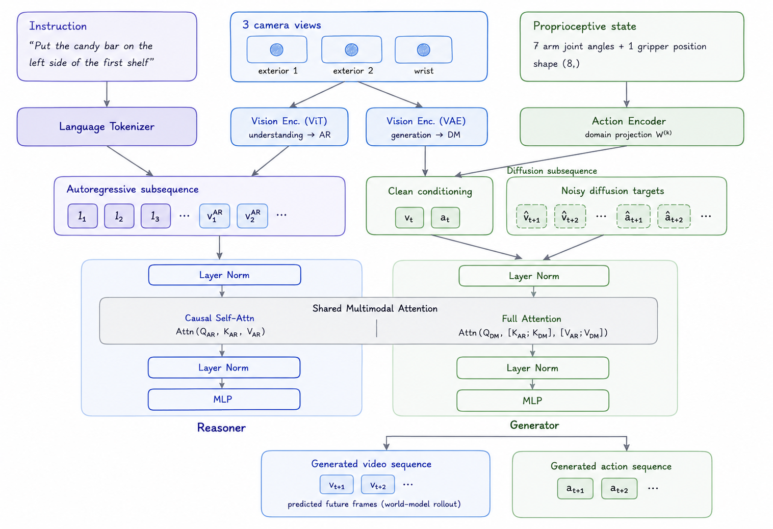
Each input is first transformed into a numerical representation and packed into two subsequences. The autoregressive subsequence contains text and image tokens. The Reasoner processes these tokens in a parallel prefill with a causal attention mask; causal attention does not mean that the supplied prompt is processed one token at a time.

The diffusion subsequence contains image and action representations together with noisy video and action targets. The Generator denoises these targets over several steps while attending to the Reasoner's representations.

The serving interface exposes the two-tower pipeline as one policy request that returns an action sequence.

How Attention Sharing Works

The Reasoner and Generator are connected inside every transformer layer. Each Reasoner layer passes its keys and values to the Generator layer at the same depth.

The Reasoner first performs causal self-attention over the instruction and image tokens:

Each Reasoner layer then exposes its key and value tensors:

The Generator creates its own queries, keys, and values from the packed video-and-action sequence. Before attention runs, the keys and values from the matching Reasoner layer are prepended to the Generator's own keys and values:

The Generator then performs one full, non-causal attention operation:

In the end, the queries come only from the Generator. Each image or action token can, therefore, attend to:

• the understanding context (instruction and image) produced by the Reasoner,
• the image tokens in the Generator sequence, and
• the action tokens in the Generator sequence.

Instruction conditioning, image-to-action interaction, and action-to-action interaction all happen in the same attention operation. There is no separate fusion module or additional cross-attention stage for each modality.

The logic is illustrated below:

# Run the Reasoner once and keep one K/V pair per layer.
reasoner_cache = reasoner(instruction_tokens, camera_image)

# Reuse that understanding context during every denoising pass.
for denoising_step in unipc_steps:
    for generator_layer, (k_reasoner, v_reasoner) in zip(
        generator_layers,
        reasoner_cache,
    ):
        # Project the packed video-and-action sequence.
        q_generator, k_generator, v_generator = (
            generator_layer.project(generator_hidden)
        )

        # Add the understanding context from the matching Reasoner layer.
        k_all = torch.cat([k_reasoner, k_generator], dim=1)
        v_all = torch.cat([v_reasoner, v_generator], dim=1)

        # Attend jointly to instruction, image, video, and action tokens.
        generator_hidden = generator_layer.attention(
            q_generator,
            k_all,
            v_all,
            causal=False,
        )

The Reasoner processes the instruction and image and produces one cached key/value pair for every transformer layer. The Generator reuses that fixed understanding context while repeatedly denoising the video and action sequence.

This is different from ordinary LLM serving. An autoregressive LLM grows its KV cache as it emits new tokens. Cosmos 3 instead keeps the Reasoner cache fixed and reruns full, non-causal Generator attention at every denoising step. The serving system must, therefore, coordinate one instruction prefill with several Generator passes for each request.

The Cosmos3-Nano-Policy-DROID model can run directly in native PyTorch, which is the simplest option for local experiments or a single robot. Upstream vLLM alone is designed primarily for autoregressive language models; it does not orchestrate this combined autoregressive and diffusion policy pipeline. I chose vLLM-Omni because it keeps the vLLM serving interface and allows adding the diffusion engine and Cosmos-specific pipeline.

The Architecture Behind the Endpoint

In my implementation, starting vllm-omni serve <model> --omni launches the FastAPI server, the asynchronous orchestrator, and a single GPU worker running the complete Cosmos 3 policy pipeline. There is no network boundary between the Reasoner and Generator. Both live inside the same GPU worker and exchange tensors directly.

client
  │
  │ POST /v1/videos
  ▼
FastAPI API server
  │
  ▼
AsyncOmni orchestrator
  │
  ▼
one Cosmos 3 GPU stage
  ├── optional guardrails and robot-observation preprocessing
  ├── camera encoding with the Wan VAE
  ├── Reasoner instruction prefill
  ├── repeated Generator denoising passes
  └── action projection and postprocessing
  │
  ▼
[32, 8] action chunk

Request and Response Flow

Each replay observation is sent as a multipart POST /v1/videos request. The request contains the camera frame, the instruction, the current joint and gripper state, and the diffusion settings. It also includes policy-specific parameters such as the robot domain, action dimension, and requested action-chunk length.

POST /v1/videos  # multipart/form-data

input_reference = concat_view.png  # uploaded PNG file
model = "nvidia/Cosmos3-Nano-Policy-DROID"
prompt = instruction
num_frames = 32
num_inference_steps = 4
guidance_scale = 3
flow_shift = 5
seed = seed

extra_params = json.dumps({
    "action_mode": "policy",
    "domain_name": "droid_lerobot",
    "action_chunk_size": 32,
    "raw_action_dim": 8,
    "robot_obs": {
        "prompt": instruction,
        "observation/joint_position": joint_position,
        "observation/gripper_position": gripper_position,
    },
})

The initial request returns a job identifier. The client then polls GET /v1/videos/{id} until inference is complete. The final response contains the generated [32, 8] action chunk: 32 future timesteps, each with seven joint-position values and one gripper value. The implementation also reads server timing fields such as stage_durations and inference_time_s, plus peak GPU memory when the server reports it.

I used the profiling and tracing support in vLLM-Omni to inspect the execution path. The resulting traces can be opened in Perfetto. Because profiling adds overhead, the latency values below come from unprofiled requests; after each measured pass, I ran one additional profiled request for kernel and model-stage attribution.

Measuring Latency

I ran the experiments as a serverless job on one NVIDIA H100 GPU provided by Nebius Cloud. The client and vLLM-Omni server ran within the job, and latency was measured from submitting one observation to receiving its complete 32-action chunk. I organized it as a cumulative waterfall. Each configuration keeps the changes from the preceding one, so the difference between adjacent bars estimates the incremental effect of the newly added technique.

The configurations are:

• E0 — baseline: BF16 eager execution with the diffusion tower explicitly forced to the TORCH_SDPA attention backend.
• E1 — FlashAttention: switches that backend to FLASH_ATTN, reducing attention latency by avoiding materialization of the full attention matrix and cutting GPU memory traffic.
• E2 — torch.compile: fuses small elementwise and normalization operations into larger kernels, reducing intermediate memory traffic and kernel-launch overhead.
• E3 — CUDA graphs: enables graph capture and replay for graph-eligible execution in the autoregressive tower, reducing CPU launch overhead. The vLLM-Omni version used here does not expose an equivalent diffusion-tower CUDA-graph switch.
• E4 — FP8 quantization: requests dynamic FP8 execution for supported kernels, reducing memory traffic and accelerating Tensor Core operations. This is an experimental, lossy configuration that requires a separate policy-quality gate.

This is a shorter list than is common in mature LLM serving stacks. Diffusion inference is still an active optimization area: the literature covers faster samplers, step distillation, feature caching, compression, and diffusion-specific serving systems, as summarized in this survey of efficient diffusion models. These methods are promising, but they are not yet drop-in, validated options for this Cosmos policy and vLLM-Omni serving path. I, therefore, limited the waterfall to techniques that could be applied and measured reliably in this setup.

Moreover, this benchmark focuses on batch-one latency for one robotics-policy request where images are conditioning inputs, and the output is a [32, 8] action chunk. Many diffusion optimizations instead target high-resolution media generation, concurrent batching, or multi-GPU throughput. Cache-DiT was tested, but it consistently increased latency. With only four denoising steps, the technique does not provide a significant benefit ( vLLM documentation). Batching and distributed parallelism were outside this one-request, one-H100 latency study.

For every configuration, I discarded 50 warm-up requests and then measured 50 requests at batch size one. Each measured request used a different observation from the DROID dataset used to post-train the Cosmos3-Nano-Policy-DROID checkpoint.

The same 50 samples, model weights, sampling settings, hardware, and software environment were used throughout. The request seed was fixed per sample. The plots report the median, with 95% bootstrap confidence intervals where error bars are shown.

Results

The first two plots summarize the unprofiled latency measurements. The last two use the separate profiling traces to explain the GPU work.

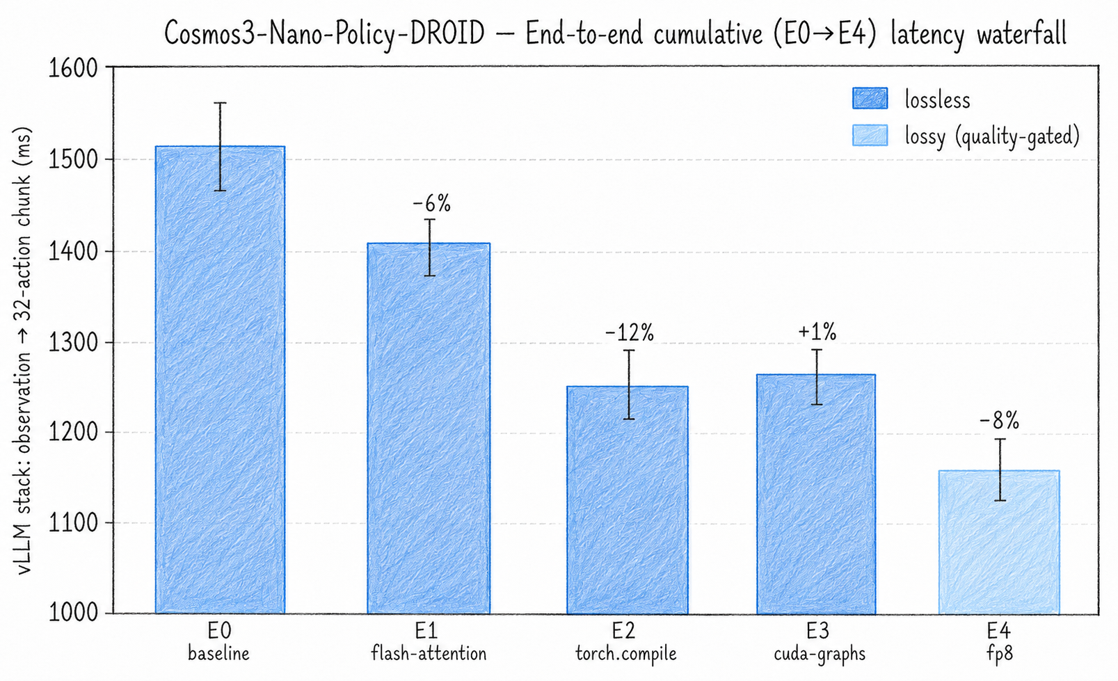
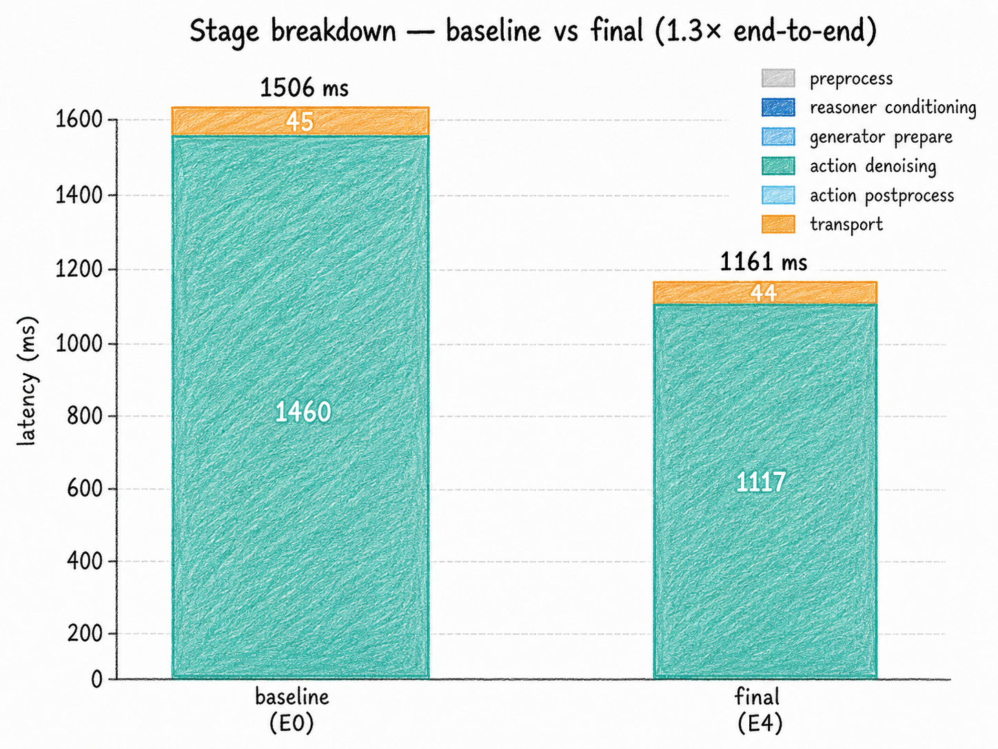
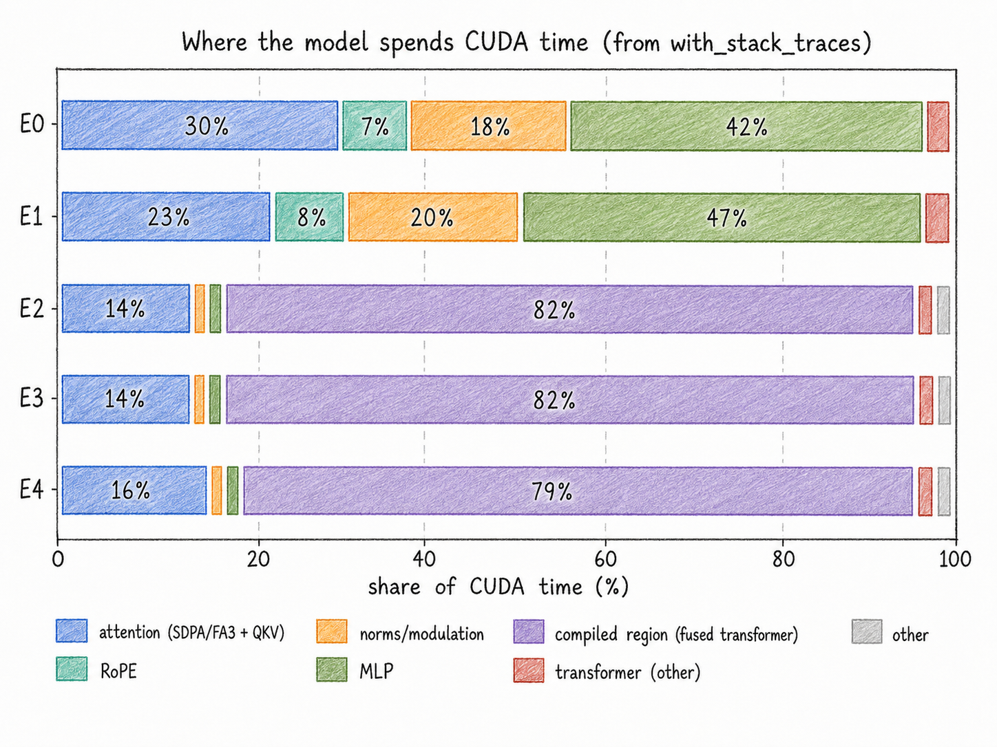
E1 cuts latency by about 6% with FlashAttention. The gain is moderate because attention is only one part of each transformer block.

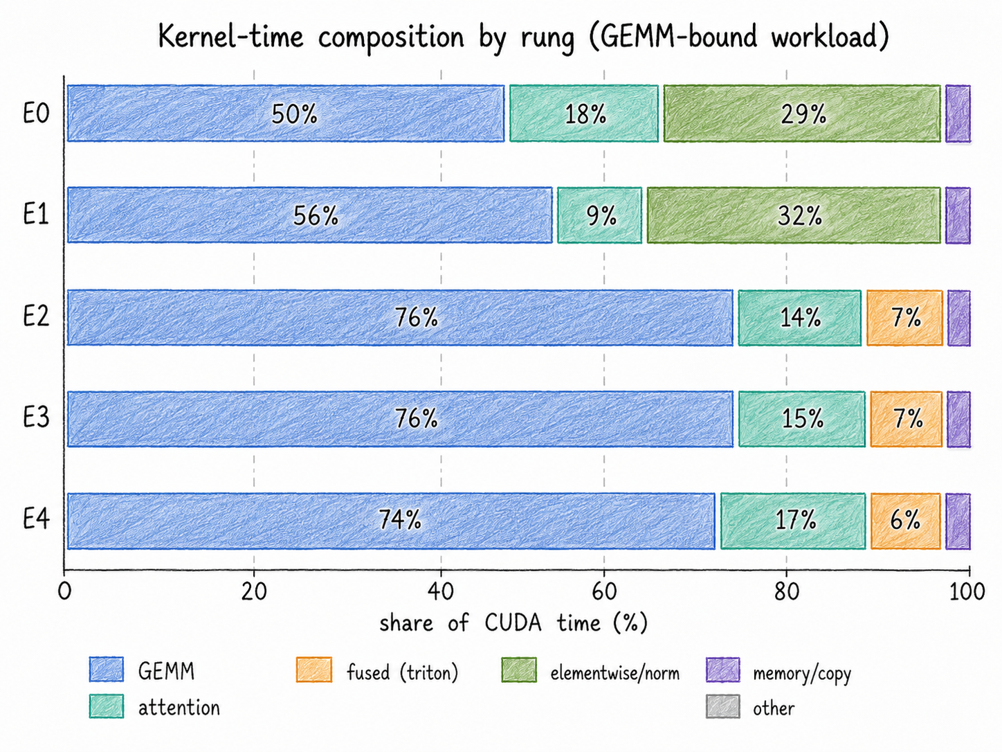
E2 delivers the largest gain, cutting another 12%. torch.compile fuses elementwise and normalization work that previously consumed 29–32% of CUDA time. MAtrix multiplication operations (GEMM) consequently rises from 50–56% to about 76% of a shorter run: its share grows because surrounding overhead shrinks.

E3 is effectively flat and about 1% slower than E2. It adds graph selection and other overhead to the graph-eligible autoregressive path. Those costs are worthwhile when CPU kernel launches are a bottleneck, but that is not the case here: most request latency comes from large denoising kernels in the diffusion tower, where this configuration does not enable CUDA graphs.

E4 adds experimental FP8 quantization, reducing latency by another 8% to 1,161 ms. Where FP8 is supported, weights use 8 bits instead of 16, so roughly half as many bytes must be loaded and moved through GPU memory for computation. FP8 also enables faster Tensor Core operations. The kernel mix remains similar—74% GEMM, 17% attention, and 6% fused Triton—showing that FP8 accelerates the dominant compute path without changing the overall execution structure. Since lower precision can alter the generated actions, this latency improvement is accepted only if E4 passes the separate RoboLab quality gate described below.

Performance Evaluation

I use RoboLab to evaluate the model performance. It is a very recent benchmark: the RoboLab paper was released in April 2026, only a few months before this article. Its initial RoboLab-120 suite contains 120 manipulation tasks organized along three competency axes—visual, procedural, and relational—and three difficulty levels. Rather than reporting only an aggregate success rate, it is designed to expose where a task-generalist policy succeeds, where it fails, and how sensitive its behavior is to controlled changes in the environment.

What is particularly new is how the benchmark itself is constructed and extended. RoboLab supports both human-authored and LLM-assisted generation of scenes and tasks from reusable assets. Tasks are expressed independently of a particular policy and are scored with composable predicates over simulator state. Objects, layouts, backgrounds, instructions, and success conditions can, therefore, be combined to create evaluations for different domains without hand-building an entirely new benchmark for every policy. The robot embodiment and inference client are configurable as well, making the same task framework useful for policies served through interfaces such as OpenPI or GR00T.

This reflects a broader trend visible in both models and benchmarks. Robot models are moving from specialized policies toward generalist systems that cover more embodiments, modalities, and tasks. Benchmarks are moving in the same direction: away from small, fixed task suites and toward extensible evaluation frameworks.

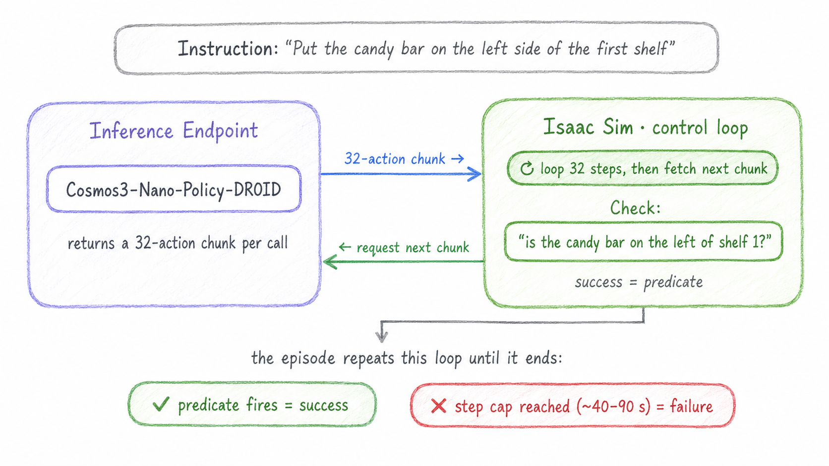
RoboLab runs on Isaac Lab, NVIDIA's robot-learning framework built on Isaac Sim, which supplies the physics, rendering, and task environments. The simulator and model run on separate machines: rendering uses an RT-core GPU, while inference uses the H100 endpoint.

Automated success detection uses a predicate: a true-or-false test on the simulator's ground-truth scene state, such as “is the candy bar on the left of shelf 1?” The endpoint and simulator interact until the predicate becomes true or the task's step cap is reached. A fair comparison also requires the same task definitions, initial-state distribution, seeds, simulator version, instructions, and number of episodes for both policies.

Unfortunately, just before the submission deadline, all instances were unavailable to run the evaluation jobs. You can do it yourself (which is almost always the best approach) for one of the configurations and compare with the performance of the quantized model. The job and endpoint creation pipelines are available in the project repository.

Conclusion

Diffusion is the most expensive part of this policy. The Reasoner conditions the request once, while the Generator repeatedly runs large transformer blocks across four denoising steps to produce one action chunk and those repeated passes are dominated by matrix multiplication.

The next gains must, therefore, reduce or reuse denoising work. Promising directions include faster samplers, fewer-step distillation, feature caching, and diffusion-specific scheduling—techniques and most of them still need to be tested for policy quality and integrated into the vLLM-Omni serving path. This experiment measured one-request latency; the next systems step is load testing to understand throughput, queueing, and tail latency under concurrent robot requests. Moreover, additonal latency reduction techniques such as multi-gpu parallelism can be exploited in more complex experiment setups.

Robotics infrastructure itself is a challenge as it must incorporate all the multi-modal requirements. Nebius Physical AI that was used to provision the GPU resources for the experiments is an actively developed project that aims to reduce this infrastructure burden significantly.

There is still much to test and explore. Happy experimenting!