Everyone wants to pay less and get more.
Benjamin Graham, in his legendary work The Intelligent Investor, wrote that speculative trading turns unintelligent in exactly three situations: when you think you're doing something else entirely, when you do it seriously without the knowledge to back it up, and when you risk more than you can afford to lose on a bad guess.
Speculative decoding plays by the same rules. It is a way to make large language models generate text faster — without changing the model architecture, without renting additional GPUs. When the conditions are right, the gains are significant: several times faster inference, with no degradation of performance. When they are not, you pay for the bet without collecting the reward.
This article is about getting the conditions right — what speculative decoding actually is, why it works, and how to know which side of it you're on.
Key problem: the next-token generation is slow
A transformer generates text one token at a time: it produces a token, appends it to the sequence, and runs the whole network again to get the next one. Each token depends on every token before it, so the process is irreducibly serial — a hundred tokens means a hundred forward passes, each waiting on the last. The diagram below illustrates this (for simplicity a word = a token).
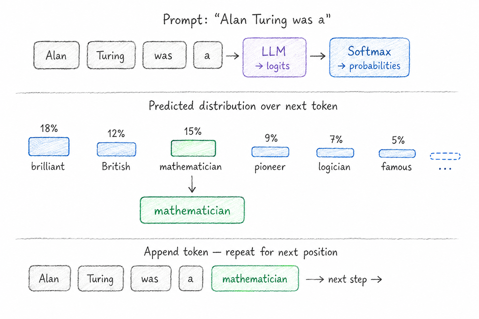
What makes each pass slow is memory, not compute. To produce a single token the model streams its entire set of parameters from memory into the chip, then does a tiny amount of arithmetic on one token's worth of activations. The arithmetic finishes in microseconds; the memory transfer takes orders of magnitude longer. Transformer decoding is memory-bandwidth bound: to a first approximation, the time per token is set by the size of the model's parameters in memory, and the chip's arithmetic units sit idle waiting for data. Pope et al. measured this directly on PaLM 540B — decode reaches roughly 14% FLOP utilization versus 76% during prefill (the stage before decode) on the same hardware (arXiv:2211.05102). The chip is not slow; it is waiting.
A 70B dense model moves all 70 billion parameters across the bus per token, one step at a time — and because each token depends on the last, a single stream can't amortize that cost across its own successive tokens (batching amortizes it across different sequences, but that doesn't speed up one stream). It is also why quantisation and distillation help — they shrink the bytes crossing the bus. Speculative decoding attacks the same bottleneck from a different angle: not by making each step cheaper, but by getting more tokens out of each step.
The bet
The whole method rests on one observation. Since a forward pass loads all the weights anyway, and the arithmetic is nearly free by comparison, the model can score not just one token but an entire candidate sequence in a single pass at almost no extra cost.
So we place a bet. Before running the expensive target model, run a much smaller, faster draft model first and let it guess the next few tokens, autoregressively and cheaply. Then feed the whole sequence — prompt plus draft tokens — through the target model in one pass. The target scores every position in parallel, comparing what it would have predicted against what the draft proposed. Where they agree closely enough, the draft token is accepted; at the first disagreement the draft token is rejected, a replacement is resampled, and everything after it is discarded.
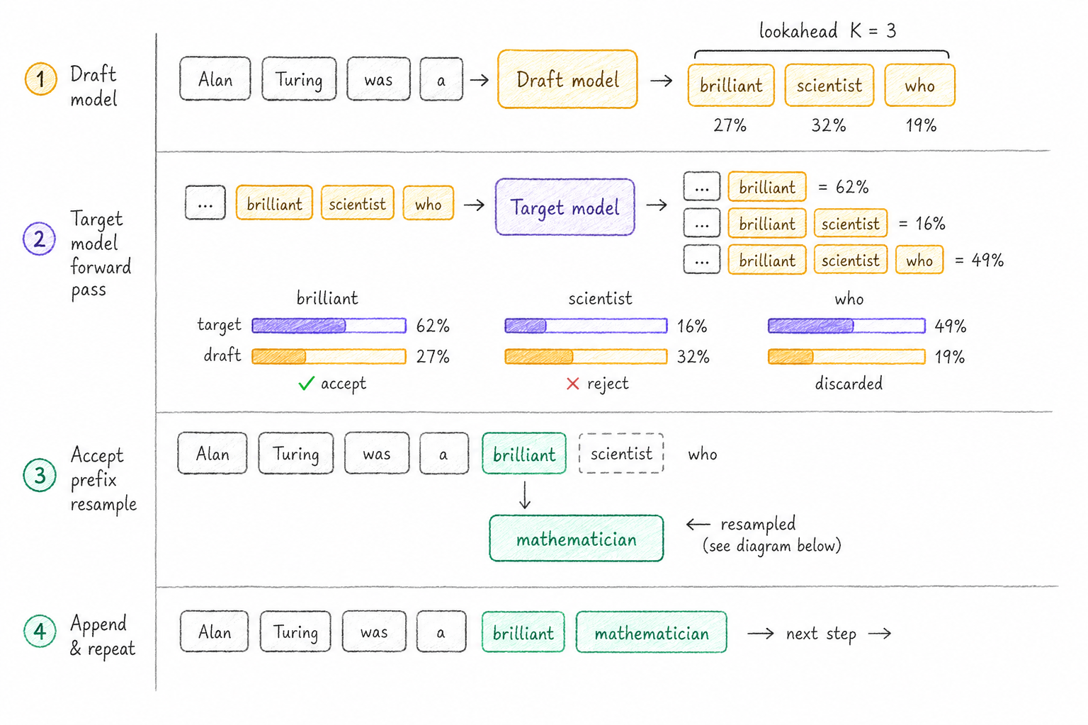
The worst case is one token — the same as ordinary decoding, so you never lose. The expected case, with a well-matched draft, is two to three tokens per target call, leading to a 2–3× speedup on average. And the output is provably identical to what the target would have produced alone. The formal algorithm is in Chen et al. (arXiv:2302.01318). Moreover, the accept–reject rule and residual resampling are built precisely so the draft's bias cancels out. The proof is short and lives in the two founding papers — Leviathan et al. (arXiv:2211.17192, Appendix A.1) and Theorem 1 of Chen et al. (arXiv:2302.01318).
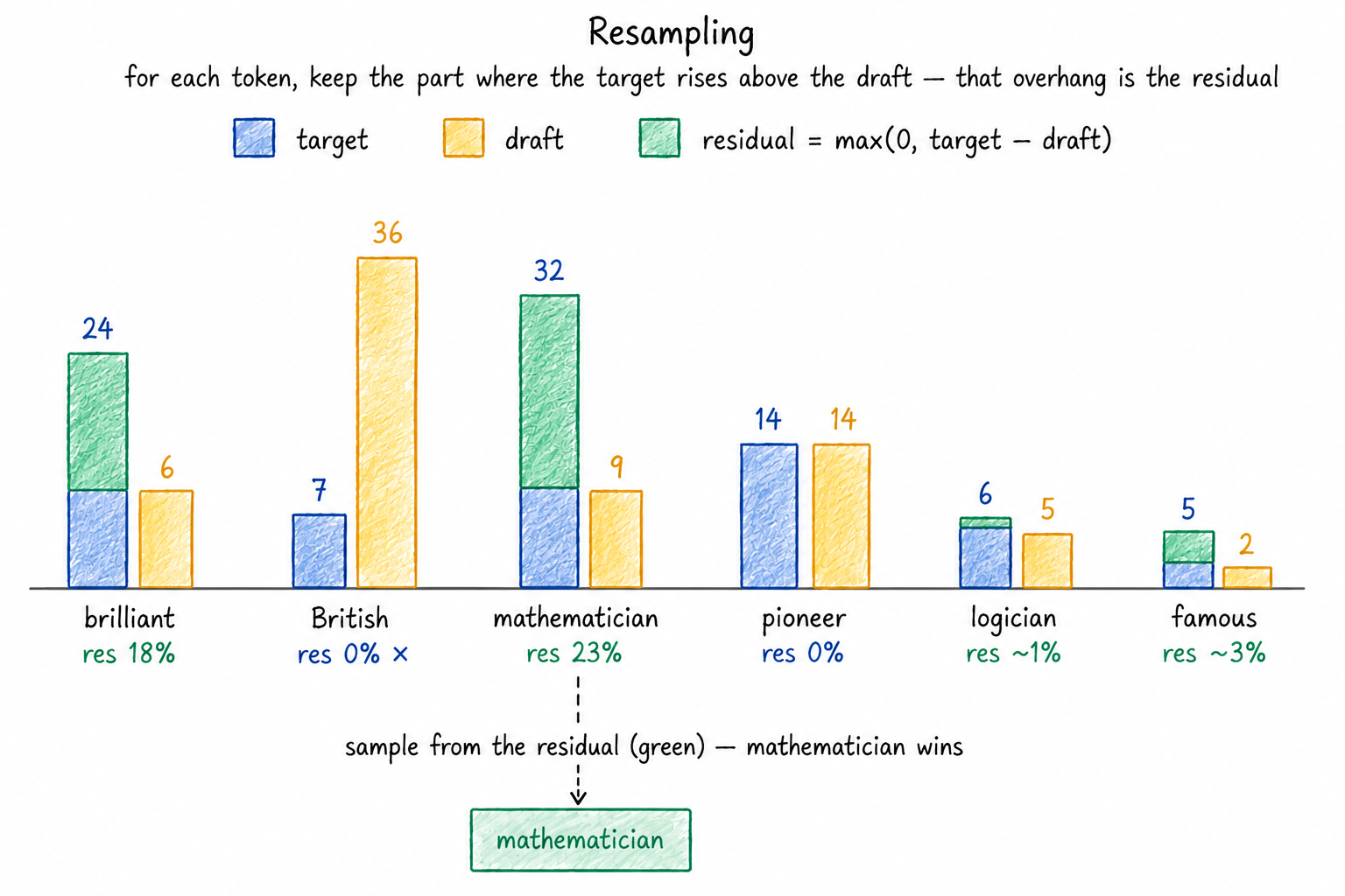
Graham would call this closing the position cleanly :) The speculative bet is fully hedged — you capture the upside when the draft is right, and when it's wrong, the correction mechanism ensures you pay nothing extra for the mistake.
Choosing the lookahead K and the draft model
Two knobs decide whether the bet pays off: the lookahead K (how many tokens the draft guesses) and the acceptance rate α (the fraction of draft tokens the target keeps). Leviathan et al. give the wall-clock speedup in closed form:
The theoretical estimation tells the story:
| acceptance α | lookahead K | extra operations | speedup |
|---|---|---|---|
| 0.6 | 2 | 1.53× | 1.96× |
| 0.7 | 3 | 1.58× | 2.53× |
| 0.8 | 2 | 1.23× | 2.44× |
| 0.8 | 3 | 1.63× | 3.69× |
| 0.9 | 2 | 1.11× | 2.71× |
| 0.9 | 10 | 1.60× | 6.86× |
Turned into design rules:
- Better draft leads to higher acceptance rate (α), but higher c. A better draft is usually a larger model and it guesses like the target more often (acceptance α goes up), but it also costs more per step (c goes up), and a high c eats the gain directly. The sweet spot is a draft roughly two orders of magnitude smaller than the target — enough to guess well, cheap enough to stay negligible.
- Raising α beats raising K. Acceptance is the dominant lever — the speedup climbs steeply with α but only gently with K. Spend effort on a better-matched draft before reaching for more lookahead.
- Set K to match your α. High acceptance justifies deep lookahead; low acceptance does not. At α = 0.9, K = 10 still pays off; at α = 0.6, K past 2–3 is wasted. Predictable domains like code push α up and reward larger K; open-ended prose keeps α modest, so keep K small.
- You have to measure α. The theory can't hand it to you — it depends on the draft–target pair, the domain, and even temperature. Run the pair over a representative sample of real traffic, count the fraction of draft tokens accepted, and use that α to choose K.
Medusa: when the model drafts for itself
The biggest practical headache in speculative decoding is the draft model itself: you must find or train a small model that matches the target, keep it aligned, and serve a second network alongside the first. Medusa (arXiv:2401.10774) does not need a draft model — the target model drafts for itself.
For every position, a transformer's last layer produces a hidden state: a vector summarising everything the model "knows" at that point. Normally a single output layer — the language-model head — turns that vector into the next token. Medusa adds a few extra heads, each a single small feed-forward layer that reads the same hidden state. What distinguishes them is what each is trained to predict: head 1 predicts the token one position ahead, head 2 the token two ahead, and so on — about five heads, each a separate learned layer specialising in its own offset. Because every head reads the target's own hidden state, its guesses stay aligned with the target's distribution, and because each is just one layer, serving stays simple.
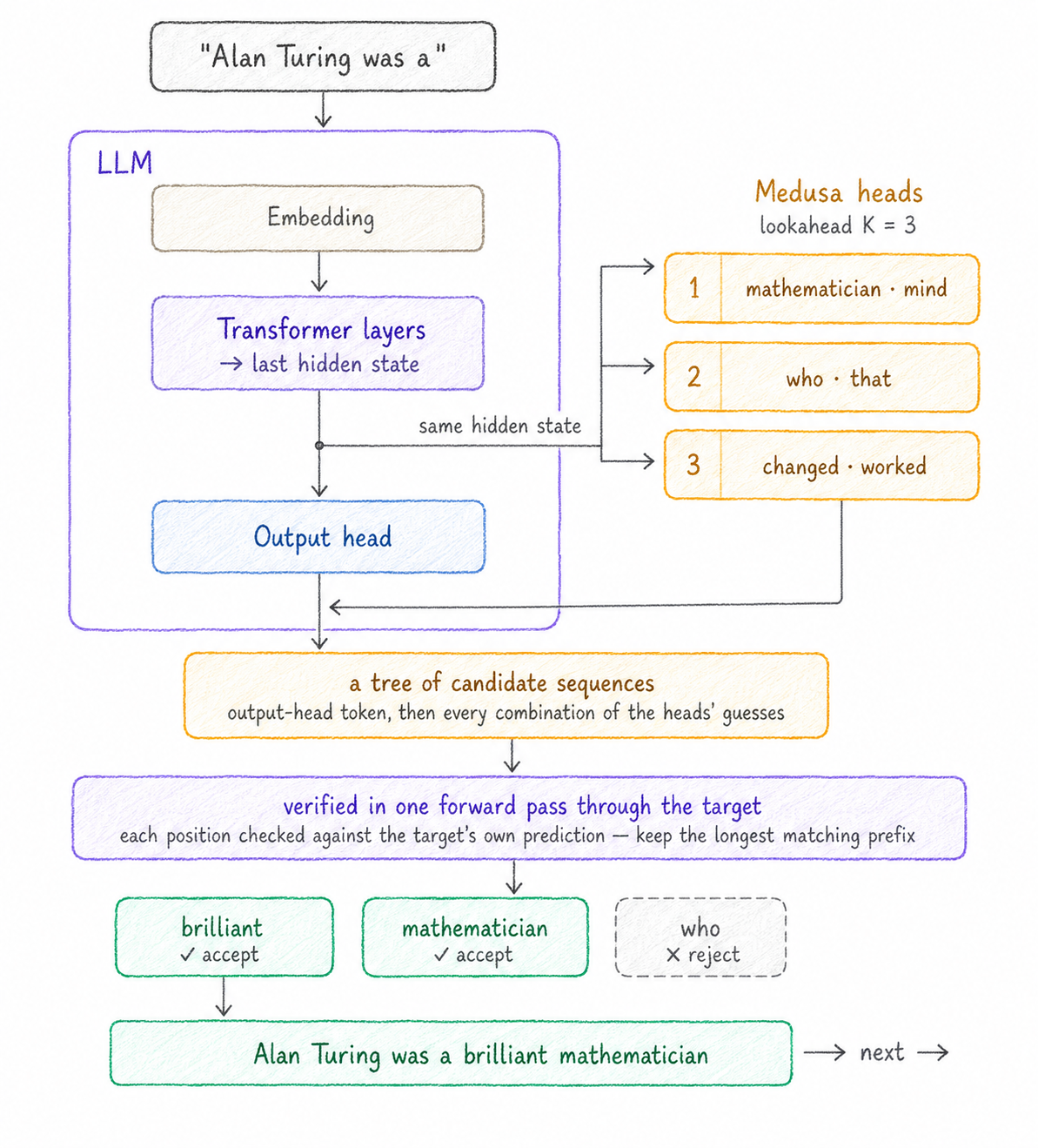
Each head offers a few candidates rather than one, so the guesses form a small tree of continuations, which Medusa checks in a single target pass. It keeps the longest branch the target accepts, then repeats — and prunes the tree toward the branches most likely to be accepted, so a small well-chosen tree beats a much larger one.
The heads do have to be trained, and Medusa offers two recipes. Medusa-1 trains only the new heads on top of a frozen target model. Medusa-2 trains heads and target model jointly for higher acceptance, which needs more care to protect the target's own quality. Medusa-1 reaches about 2.2× and Medusa-2 roughly 2.3–2.8× on Vicuna, with the largest gains — over 3× — on predictable domains like code and extraction.
EAGLE: drafting on features, not tokens
Medusa cuts the draft model out; the EAGLE line takes the opposite bet — keep a draft, but make it a far better guesser by feeding it richer information. The result is the strongest lossless speculative decoding family in wide use, and it arrived in three steps.
EAGLE-1 (arXiv:2401.15077) rethinks what a draft should work from. An ordinary draft model re-derives its understanding of the context from scratch — a poorer representation than the one the target has already computed. EAGLE's insight is to skip that waste: reuse the target's own features — the hidden states it computes anyway during prefill and verification.
Therefore, the drafter becomes just a single transformer layer — not a whole separate model — trained for this target that predicts the target's next feature, then maps that feature to a token through the target's own output head. Training makes the correspondence explicit: a regression loss pulls the draft's predicted feature toward the target's true feature at that position, so the small layer learns to imitate one step of the big model's hidden-state trajectory. Choosing a draft, then, is not a matching problem — you simply train one lightweight layer against your target.
The one wrinkle is sampling: the next feature depends on which token was drawn, but sampling is random, so a feature alone doesn't reveal the actual draw. EAGLE, therefore, feeds the sampled token back into the draft alongside the feature, pinning down which continuation it's on before predicting the next step. Like Medusa, it drafts a tree of candidates and verifies with tree attention — though here the tree is static, fixed in advance.
EAGLE-2 (arXiv:2406.16858) makes that tree dynamic. EAGLE-1's tree has a fixed shape, which wastes effort: it spends as many candidates on hard positions (where the draft is probably wrong) as on easy ones (where it's probably right). EAGLE-2's fix is to let the draft's own confidence decide the shape. The drafter already outputs a confidence score with each guess, and those scores turn out to track the true acceptance rate closely — so EAGLE-2 grows more branches where confidence is high and stops early where it's low. Same number of candidates, spent where they'll actually be accepted, lifting the speedup to around 4×.
EAGLE-3 (arXiv:2503.01840) removes the last constraint holding acceptance back. Predicting features forces the drafter to match the target's feature vectors exactly, which limited how much it could learn from more training data. EAGLE-3 drops feature prediction in favour of predicting tokens directly, and — via a technique called training-time test, which simulates real inference conditions during training — fuses features from the target's low, middle, and top layers rather than the top alone, giving the drafter a fuller view of the target's computation. This both raises acceptance (into the 0.8–0.9 range on code and instruction-following) and unlocks a scaling law the earlier versions lacked: more training data now buys proportionally more speedup, up to about 6.5×.
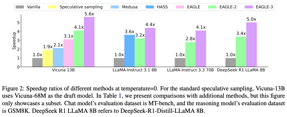
So, EAGLE-3 is the result of the approach's evolution, each version layered on the last. In practice, it's the default: it's the fastest and is merged into the major serving stacks (vLLM, SGLang, TensorRT-LLM), with pre-trained heads available for many popular models. The one reason to reach for an earlier version is cost or availability — EAGLE-1 is simpler and cheaper to train, so if no EAGLE-3 head exists for your target, it's a reasonable floor. The EAGLE line is worth a separate post, so I'll probably write about it in more depth later.
Conclusion
Speculative decoding is a genuine free lunch when it fits — two to three times faster, or more with EAGLE, at no cost to output quality.
Like any speculation, it turns unintelligent in three ways. The first is not knowing what you are actually doing. The second is doing it without the knowledge to back it up — a poorly matched drafter, a misconfigured lookahead, and so on. The third is risking more than the gain is worth — a second model to serve, or a layer and heads to train and add, especially when the model isn't very large.
Get the three right, and the bet pays off in much lower latency.