There is one operation at the heart of deep learning: matrix multiplication (GEMM). In a typical neural network, the vast majority of compute time on a GPU is spent on matrix multiplications; everything else — adding biases, normalising, applying activations — is rounding error by comparison.
The first GPU-trained deep learning model
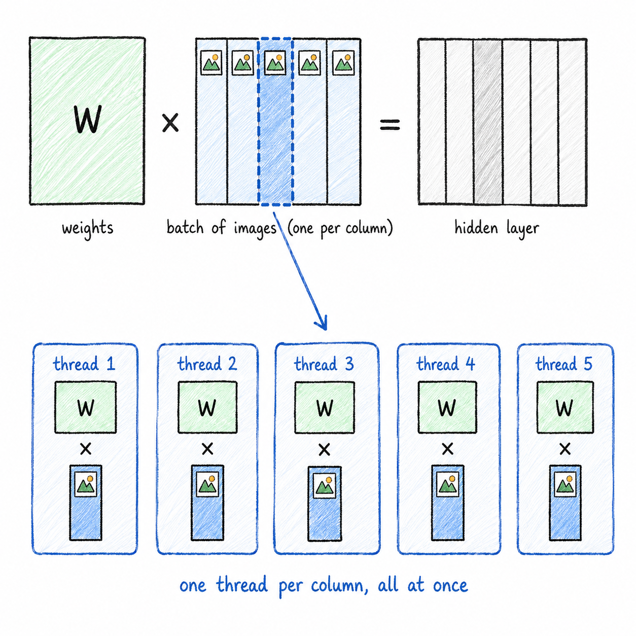
In 2009, Rajat Raina, Anand Madhavan, and Andrew Ng trained a sparse deep network on a single graphics card — an NVIDIA GeForce GTX 280 with 1 GB of memory. Their largest model, 45 million parameters, processed a million training examples in roughly 29 minutes, against more than a day on a dual-core CPU. The GPU ran 12 to 72 times faster across their experiments; the largest speedups came on the largest models, because bigger matrices expose more independent work and keep more of the hardware's cores busy simultaneously.
That 1 GB card would struggle to load a modern language model for sure. Today's training runs usually use GPUs with 80 GB (H100) or 141 GB (H200) or more of memory — and even those are not enough to hold a frontier model on a single device. However, the core insight from 2009 has not changed: each training step is a matrix multiplication, the examples in a batch are independent of each other, and the GPU is a machine built to exploit exactly that independence.
That insight scaled for a decade. However, at some point the model no longer fits in one GPU's memory — and eventually not across one node. To see where the seams are, it helps to look at exactly which operations inside a transformer carry the weight.
Where the matrix multiplications live in a transformer
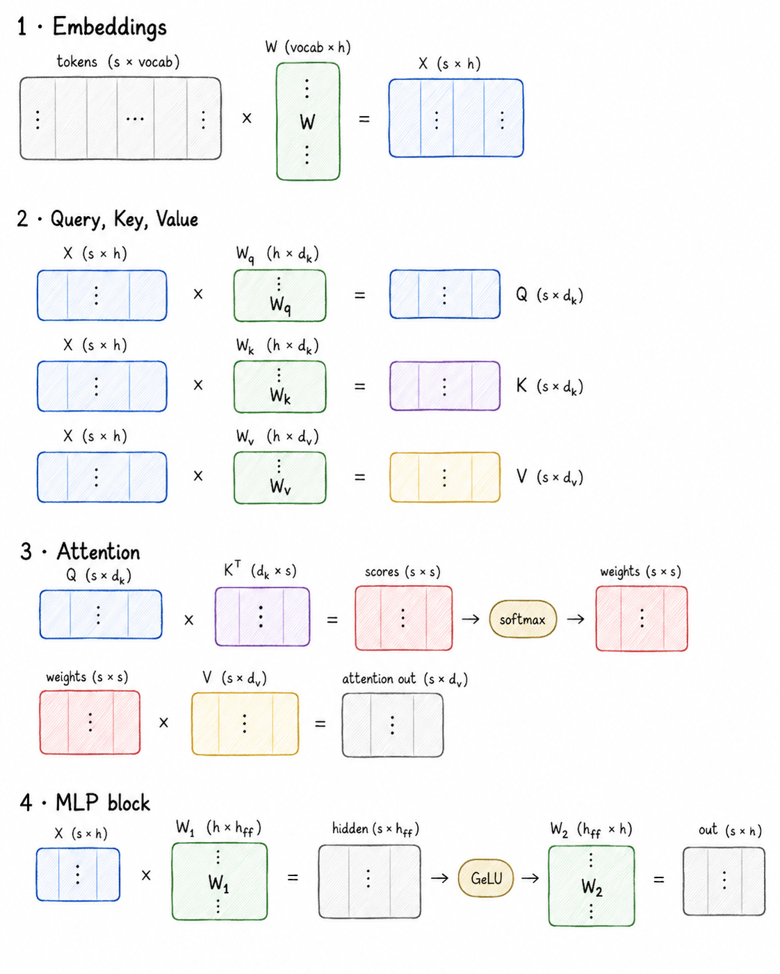
When you feed a prompt to your favourite model provider API, at the backend it is first tokenised and then sent to the model. From that point, matrix multiplication shows up at every stage. The tokens are turned into vectors by multiplying against an embedding weight matrix. Those embeddings are projected three ways — into queries, keys, and values — by three more weight matrices. Attention itself is two matrix multiplies: queries times keys to score every pair of tokens, then those scores times the values. Finally the MLP block expands and projects with two more.
A transformer layer has two blocks:
- Self-attention. The embedding matrix X is projected into queries, keys, and values by three weight matrices Wq, Wk, Wv. Attention scores are computed as a matrix product of Q and Kᵀ, passed through a softmax, then multiplied by V to produce a weighted sum. A final output projection closes the block.
- MLP block. The result is multiplied by a weight matrix W₁ that expands it to roughly four times the hidden size, passed through GeLU, then multiplied by a second weight matrix W₂ that projects it back down — two GEMMs around one cheap activation. In the tensor parallelism section below, W₁ and W₂ are referred to as A and B respectively.
Everything else — layer normalisation, softmax, residual additions — is element-wise and costs little.
Two forms of independence in this structure make it parallelisable:
- Across examples. Different sequences in a batch pass through the weights independently — the axis data parallelism exploits.
- Across the weight matrices. Each GEMM can be partitioned column- or row-wise, and attention is additionally independent across its heads — the axis tensor parallelism exploits.
Data parallelism: the batch across many accelerators
The 2009 experiment processed a million examples in 29 minutes on a single card. Today's frontier models are trained on trillions of tokens — a dataset so large that even at full GPU speed, a single device would take decades to process it. The answer is the same as it was in 2009: spread the examples across many parallel workers — threads within a GPU then, GPUs across a cluster now.
Learning is a gradient computation. The model runs a batch of inputs forward through its weight matrices and produces predictions; a loss function measures how wrong they are. The gradient is then computed by running the chain rule backward — for every forward matrix multiplication there is a corresponding backward one, producing a signal for each weight that says how much, and in which direction, adjusting that weight would reduce the loss. An optimiser then takes a step in that direction and updates the weights. The gradient is what carries the learning signal, and it is the thing that must be shared when many GPUs train together.
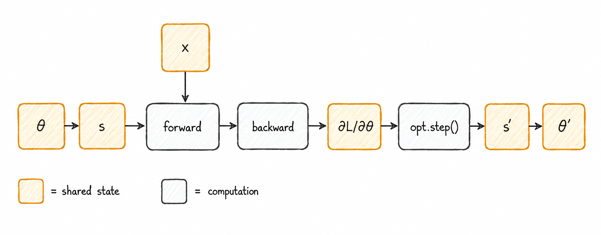
Simple data parallelism. The basic idea is direct: give every GPU a full copy of the model, assign each copy a different slice of the training batch, let them run the forward and backward passes independently, and then average the gradients across all devices before updating the weights. Since the examples are independent of each other, this is mathematically equivalent to computing the gradient on the full batch.
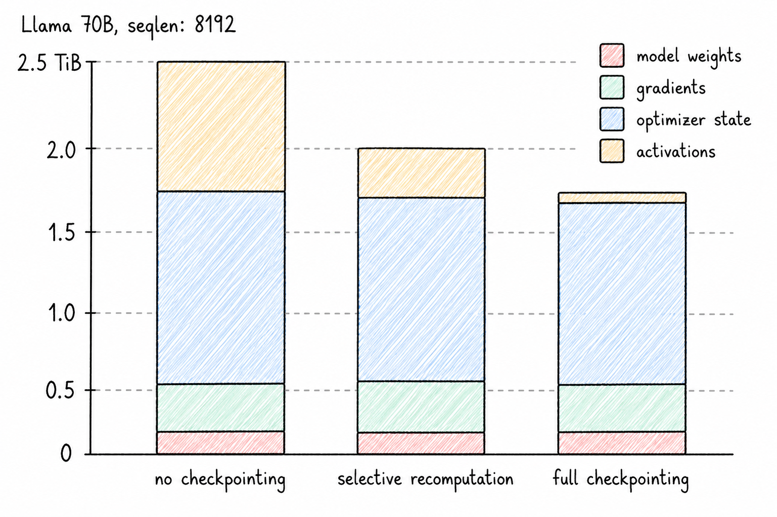
The bottleneck: every GPU holds the full model state. Simple data parallelism replicates the entire model on every device — not just the weights, but also the gradients (one derivative per weight, stored as a tensor of the same shape) and the optimiser state. For mixed-precision training with Adam, the total memory per parameter breaks down as: 2 bytes for the fp16 weight, 2 bytes for the fp16 gradient, and 12 bytes for the Adam optimiser state (a fp32 master copy of the weight at 4 bytes, plus 4 bytes each for the first and second moment estimates) — 16 bytes per parameter in total. For a model with 70 billion parameters, that is over 1 TB per device. The optimiser state alone accounts for 12 of those 16 bytes, making it by far the largest component. And every GPU holds an identical copy of all of it.
FSDP: sharding the redundancy away. The Zero Redundancy Optimiser (ZeRO, Rajbhandari et al., arXiv:1910.02054, 2020) solved this by partitioning model state across devices rather than copying it. PyTorch's implementation for that is Fully Sharded Data Parallel (FSDP, Zhao et al., arXiv:2304.11277, 2023). Instead of every GPU holding all the weights, each GPU holds only its own shard — a contiguous slice of the parameters, gradients, and optimiser state, so the total memory per device drops proportionally to the number of GPUs.
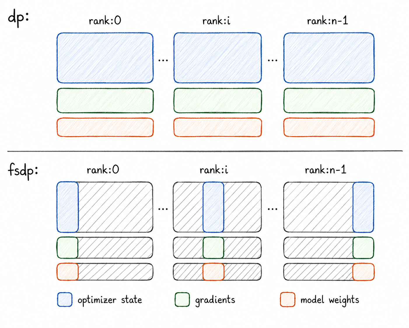
The cost is that a device no longer has the weights it needs for a forward pass. FSDP recovers them on demand: just before a layer is computed, the devices collectively assemble the full weight tensor from their shards, run the computation, and immediately discard the non-local parts. The same happens in the backward pass, after which each device retains only its own gradient shard.
However, there is a limit to what sharding storage can achieve. FSDP reduces memory, but it does not reduce the compute cost of each layer — every device still runs the full matrix multiplication for its reconstructed shard. For the largest models, that is not enough: you want the multiplication itself to be distributed across devices, so that each device only ever computes a fraction of each layer. That is what tensor parallelism addresses.
Tensor parallelism: partitioning the weights
The key is a structural property of matrix multiplication: a matrix product can be partitioned, and the way you partition it decides whether the work splits cleanly or forces the machines to coordinate.
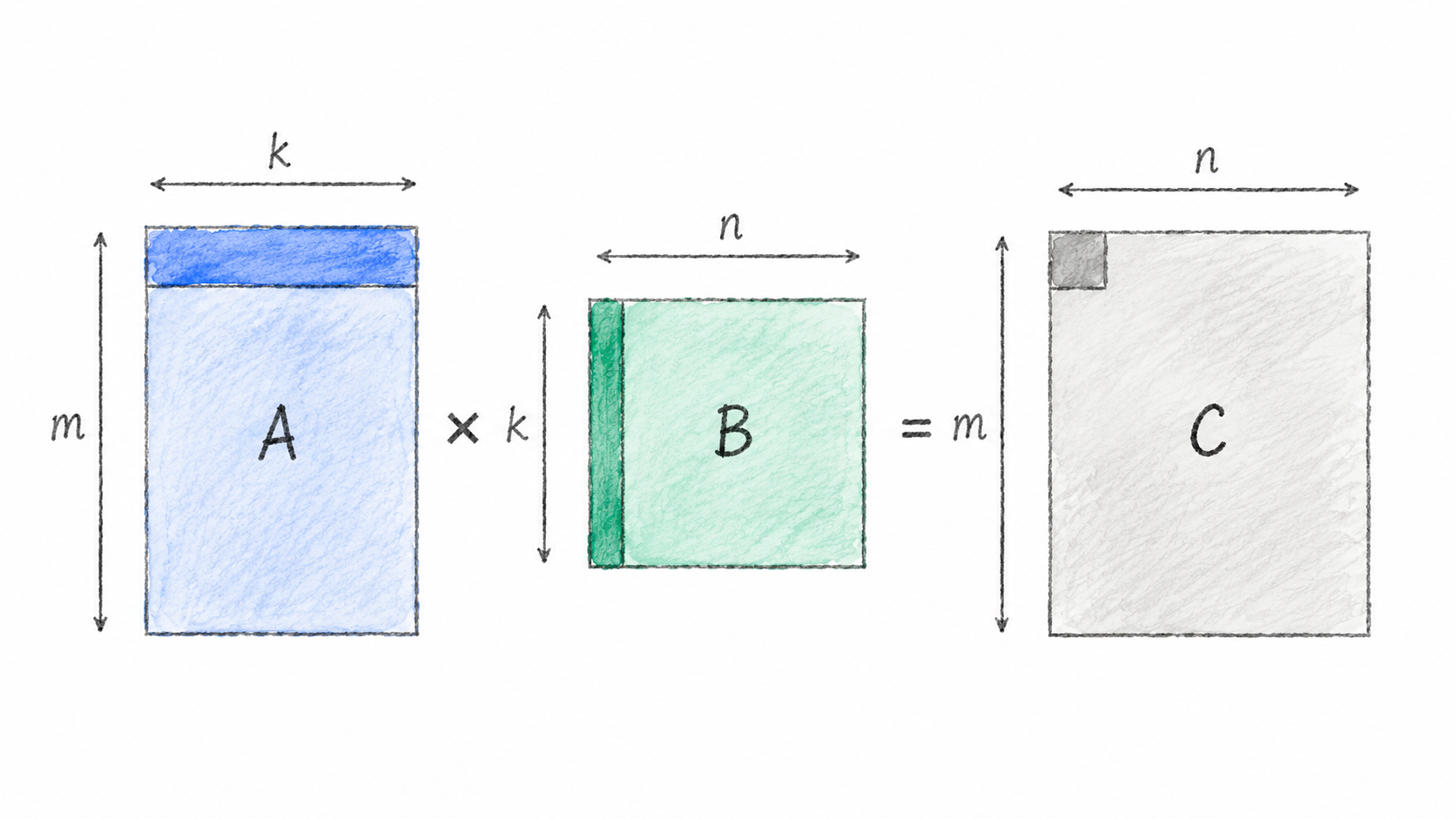
Consider the product AB where A is m×n and B is n×k. The very same product can be read three equivalent ways — and each reading is a different way to divide the work among processors.
![A in ℝ^(m×n) and B in ℝ^(n×k), with the product AB written three equivalent ways: the column-wise view AB = [Ab₁, …, Ab_k]; the row-wise view stacking the rows αᵢᵀB; and the outer-product expansion AB = Σ aᵢ βᵢᵀ.](/assets/posts/maths-parallel-training/maths_parallel_training_linear_algebra.png)
The column-wise view reads the output one column at a time: column j of AB is just A times column j of B. Each output column depends only on its own column of B, so different processors can own different columns of B and never need to coordinate with each other.
The row-wise view is the mirror image: row i of AB is row i of A times B. Each output row depends only on its own row of A, so the rows are equally independent.
The outer-product view splits along the shared inner dimension n: AB = Σᵢ aᵢβᵢᵀ, a sum of rank-one matrices each covering the full output. No processor produces a finished answer alone — every one holds a partial result, and the partials must be summed. That summation forces synchronisation, and it is the cost you pay whenever you choose this partition.
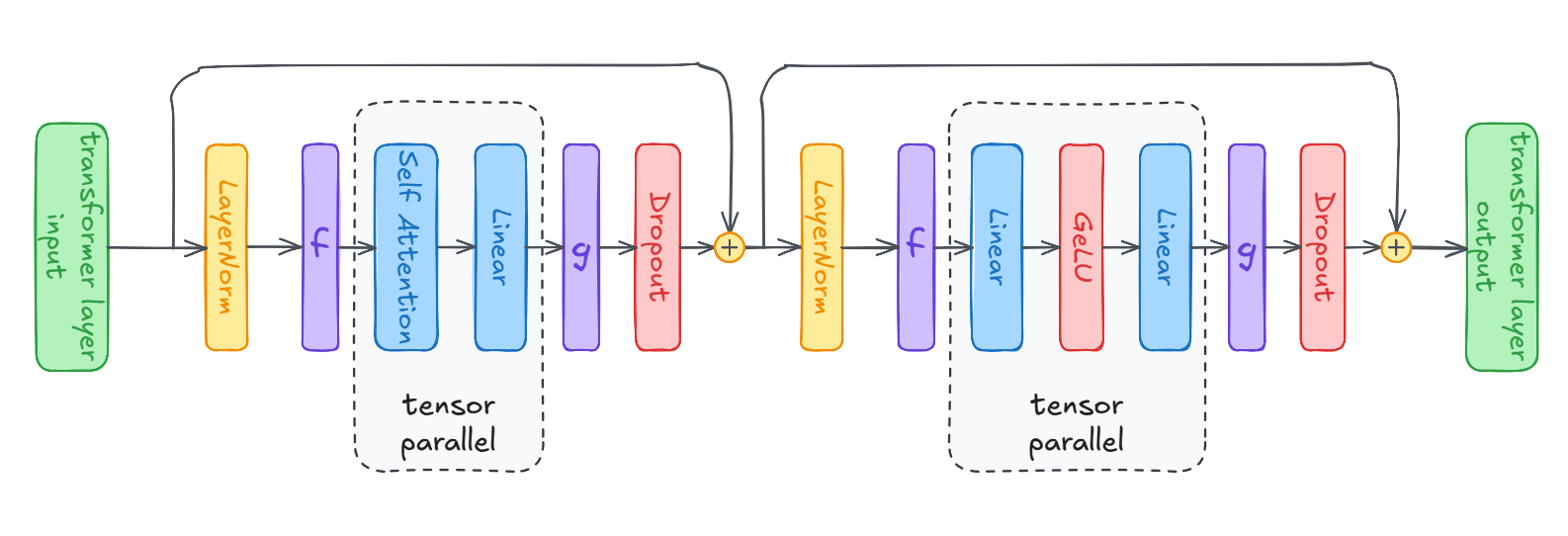
Almost all the weight in a transformer layer sits in its linear projections. The self-attention block holds the Q, K, and V projections plus the output projection; the MLP block — the second sub-layer, which follows attention — holds two further linear layers. Together these matrix multiplications account for nearly all parameters and nearly all memory. Splitting the model across devices therefore means, concretely, splitting those matrix multiplications.
NVIDIA's Megatron-LM framework formalised this in 2019 (Shoeybi et al., arXiv:1909.08053). The key insight is to use the column-wise and row-wise views of each weight matrix.
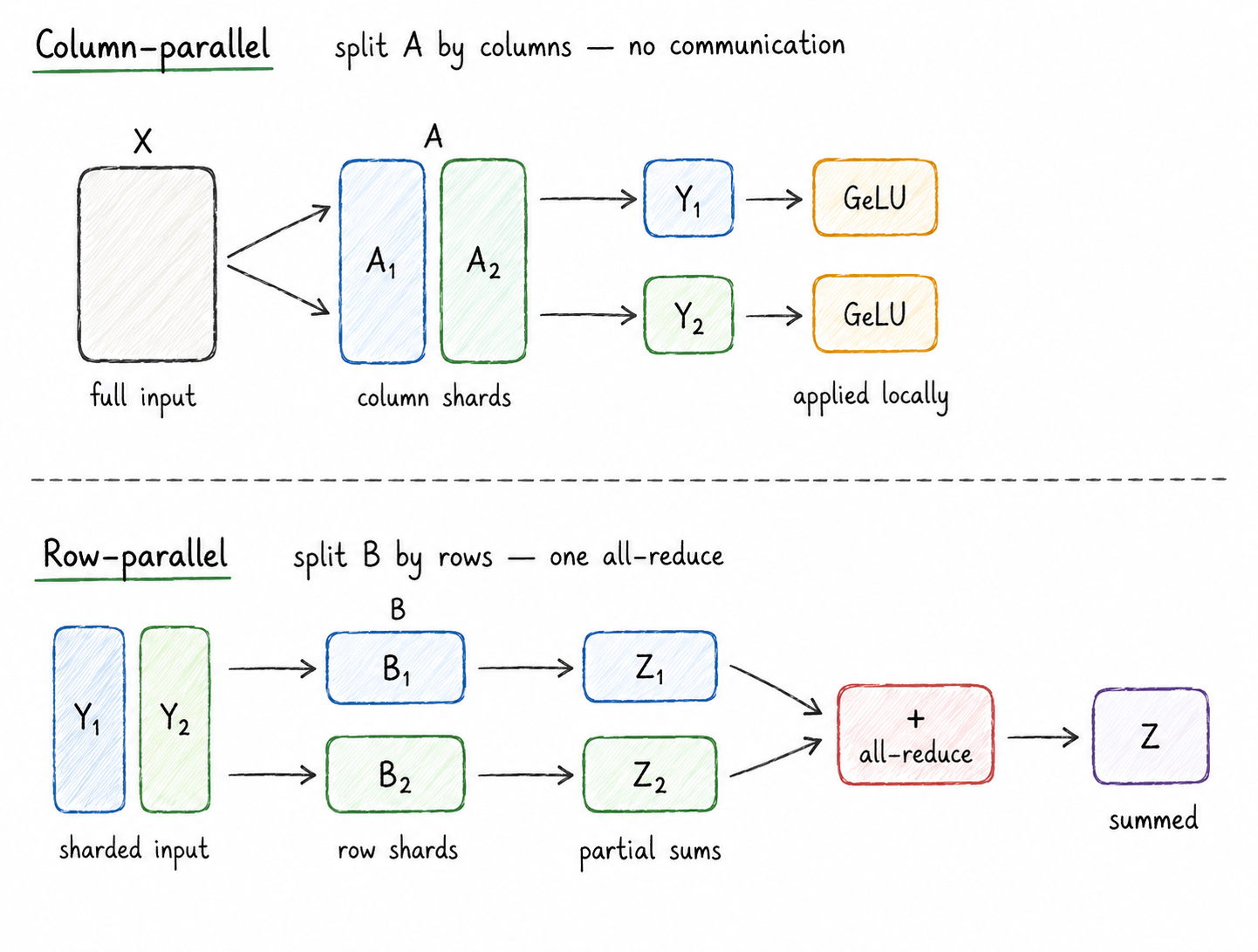
MLP block. Call the MLP block's two weight matrices A and B. The input X is multiplied by A to produce an intermediate result Y — which then passes through GeLU and is fed to B — and B produces the block's output Z. Megatron splits A column-wise and B row-wise to eliminate any synchronisation between the two projections. In a column-wise split, each device multiplies the full input matrix X against its own block of columns of A, producing the corresponding block of output columns of Y. Ordinarily, these partial outputs would need to be summed before applying GeLU — which would require a synchronisation. However, since GeLU is element-wise, each device can apply it directly to its own block of Y without ever seeing the other devices' results. B is then split row-wise to match: each device's row shard of B expects exactly the GeLU-activated Y block that the same device already holds. A single all-reduce at the end sums the partial outputs into Z.
Attention block (the same pattern). Q, K, and V matrices are each split column-wise across devices — and because multi-head attention is independent across heads, each device naturally owns a subset of complete attention heads and computes them in full, with no inter-device dependency. The output projection is then split row-wise, requiring a single all-reduce before the residual add, exactly as in the MLP block.
The result: a simple linear algebra trick reduces inter-device communication to just two all-reduces per transformer layer in the forward pass, and two in the backward — four collectives per layer, regardless of model size. This matters because inter-device communication is expensive: each synchronisation requires all devices to exchange results before computation can continue, and at scale that overhead compounds across hundreds of layers and thousands of devices.
The limitation: activation memory. Tensor parallelism needs only a few communication primitives in native PyTorch and gives roughly a t× reduction (that is, dividing memory by the number of devices t — so 8 GPUs yield roughly 8× less parameter and model-state memory) in parameter and model-state memory across t devices. What it does not shard is the layers outside the parallel blocks — layer norms, dropout, residual paths. Megatron duplicates these on every device and relies on activation checkpointing to manage their cost. As sequence lengths grow, those unsharded activations become the dominant memory cost — the problem later addressed by sequence parallelism (Korthikanti et al., arXiv:2205.05198, 2022).
Sequence parallelism
The fix is conceptually straightforward: shard the activations that tensor parallelism leaves unsharded along a dimension that is naturally independent — the sequence dimension.
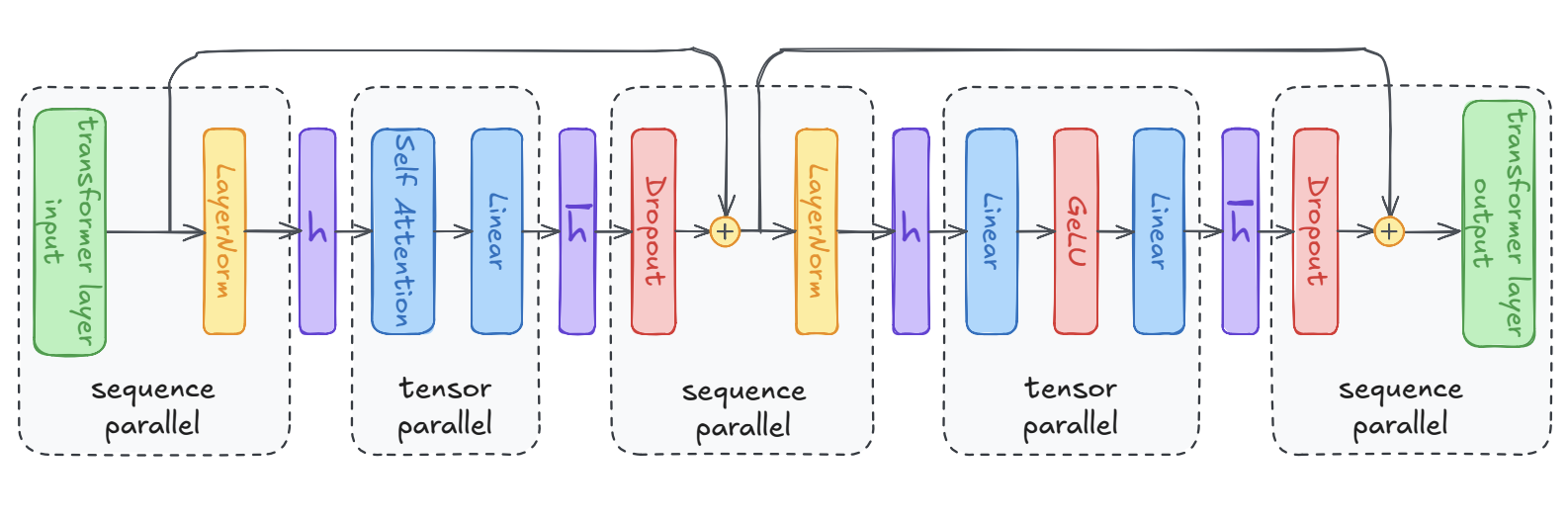
Activations are the intermediate values produced during the forward pass and retained for the backward pass. In a transformer, the tensors flowing through layer norms, dropout, and residual connections have shape (sequence length × batch size × hidden size), and tensor parallelism leaves them fully replicated on every device. As sequence lengths grow, this becomes the dominant memory cost.
Sequence parallelism splits these tensors along the sequence dimension, giving each device a contiguous slice of token positions. Layer norm is applied locally — it operates independently per token — and the slices are all-gathered before entering the next tensor-parallel block. This does not introduce additional communication overhead: an all-reduce is equivalent to a reduce-scatter followed by an all-gather, so the total bandwidth used is unchanged.
The result is a t× reduction in the activation memory of the previously unsharded regions.
When sequence parallelism is not enough
Sequence parallelism solves activation memory for moderate contexts, but as sequences grow to hundreds of thousands of tokens, attention itself becomes the bottleneck.
Context parallelism. Sequence parallelism as described above shards the non-attention activations, but attention itself still requires each device to see the full sequence when computing scores. For very long contexts — hundreds of thousands to millions of tokens — even the attention computation becomes intractable on a single device. Two approaches address this. DeepSpeed-Ulysses (Jacobs et al., arXiv:2309.14509, 2023) transposes the problem: before attention, an all-to-all collective converts sequence shards into head shards, so each device computes full attention for its own subset of heads; a second all-to-all restores the sequence layout afterward. The constraint is that the parallelism degree cannot exceed the number of attention heads. Ring Attention (Liu, Zaharia & Abbeel, arXiv:2310.01889, 2023) takes a different route: each device holds a contiguous chunk of query tokens, and key-value blocks are passed around a ring of devices while blockwise attention is computed locally — communication and computation are overlapped so the ring transfer is effectively free. Online softmax makes this exact in a single pass without storing the full attention matrix. For causal models, load balancing across ranks requires care since earlier tokens attend to fewer keys than later ones.
Expert parallelism. Mixture-of-experts (MoE) models replace the dense MLP block with a set of parallel expert networks, routing each token to a small subset (Shazeer et al., arXiv:1701.06538, 2017). Since only a fraction of experts are active per token, MoE models can scale parameter count without proportionally scaling compute. The parallelism challenge is that tokens must be dispatched to whichever device holds their assigned expert — requiring an all-to-all collective to redistribute tokens before the MLP computation and another to collect results. Expert parallelism therefore adds a new communication dimension on top of tensor and data parallelism, with load balancing across experts being a central practical concern.
Pipeline parallelism. When the model is too deep to fit across a single node's worth of tensor-parallel GPUs, pipeline parallelism assigns consecutive layer groups to consecutive device stages (Huang et al., arXiv:1811.06965, 2019). Each stage runs its layers in full and passes activations forward to the next stage. The gradient flows backward through the same pipeline during the backward pass. The key cost is the pipeline bubble — idle time when a stage waits for the previous one to finish — which is reduced by splitting each batch into micro-batches and keeping stages continuously fed. Pipeline parallelism divides model memory by the number of stages and requires only point-to-point communication between adjacent stages, making it well-suited for inter-node links where bandwidth is lower than intra-node NVLink.
Key takeaway
Every technique in this article — tensor parallelism, sequence parallelism, FSDP, pipeline parallelism and the rest — is, at its core, an answer to the same question the 2009 experiment answered on a single GPU: how do you keep as many multiplications running in parallel as possible, with as little coordination as possible?
The arithmetic itself is not the bottleneck. Modern GPUs perform matrix multiplications at close to theoretical peak. What limits scale is everything around the arithmetic: moving partial results between devices, keeping every device fed, and ensuring nothing sits idle waiting for another device to finish.